Accelerate random number generation with OpenRNG and Performix
Introduction
Set up your environment
Run the baseline data-processing example
Identify code hotspots with Arm Performix
Accelerate distribution generation with OpenRNG
Measure performance improvements with a microbenchmark
Next Steps
Accelerate random number generation with OpenRNG and Performix
Understand OpenRNG and Arm Performance Libraries
Arm Performance Libraries include numerical routines tuned for Arm processors. These Arm-tuned routines can speed up execution by reducing overhead and improving throughput for compute-heavy kernels.
OpenRNG is the random-number component in Arm Performance Libraries. It exposes a Vector Statistical Library (VSL) API, where VSL means generating distributions in vector form (many values per call) instead of one sample at a time.
You’ll use this vector API to generate Gaussian values in bulk. Bulk generation through a stream object lowers per-sample overhead, which is why this change can reduce runtime in the hotspot.
OpenRNG is API-compatible with the Intel oneMKL VSL RNG interface, so distribution call sites remain familiar when you move between x86 and aarch64 builds. You mainly switch build configuration, not workload logic. For more information, see the
OpenRNG developer reference guide
.
In src/vec1d.cpp, the USE_ARMPL macro controls which implementation is compiled. In this project, enabling USE_ARMPL selects the aarch64 OpenRNG path:
#if USE_ARMPL
    #if defined(__aarch64__)
        #include <amath.h>
        #include <openrng.h>
    #else
        #error "USE_ARMPL enabled but not on AArch64"
    #endif
#endif
The OpenRNG path creates one VSL stream and fills a contiguous buffer for both coordinates. count is 2 * v.getSize() because each point has x and y values:
VSLStreamStatePtr stream;
vslNewStream(&stream, VSL_BRNG_SFMT19937, 777);

const int count = 2 * v.getSize();
std::vector<float> tmp(count);
For Gaussian generation, the code calls the single-precision VSL routine vsRngGaussian. Here, param_a is the mean and param_b is the standard deviation:
vsRngGaussian(
    VSL_RNG_METHOD_UNIFORM_STD,
    stream,
    count,
    tmp.data(),
    param_a, // mean
    param_b  // standard deviation
);
After bulk generation, values are mapped back into your Point vector:
auto& data = v.getData();
for (int i = 0; i < v.getSize(); i++){
    data[i]._x = tmp[2*i];
    data[i]._y = tmp[2*i+1];
}

vslDeleteStream(&stream);
Build and run the accelerated variant
Build and run the accelerated variant by passing -DUSE_APL=1 to enable the OpenRNG path in vec1d.cpp:
make clean
cmake -S . -B build -DUSE_APL=1
cmake --build build --target main_with_apl
./build/src/main_with_apl
Analyze the flame graph
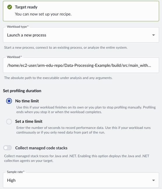
Now profile the accelerated binary in the Arm Performix GUI using ./build/src/main_with_apl as the workload. Follow the same steps as the previous section.
When the run completes, Performix displays the flame graph:
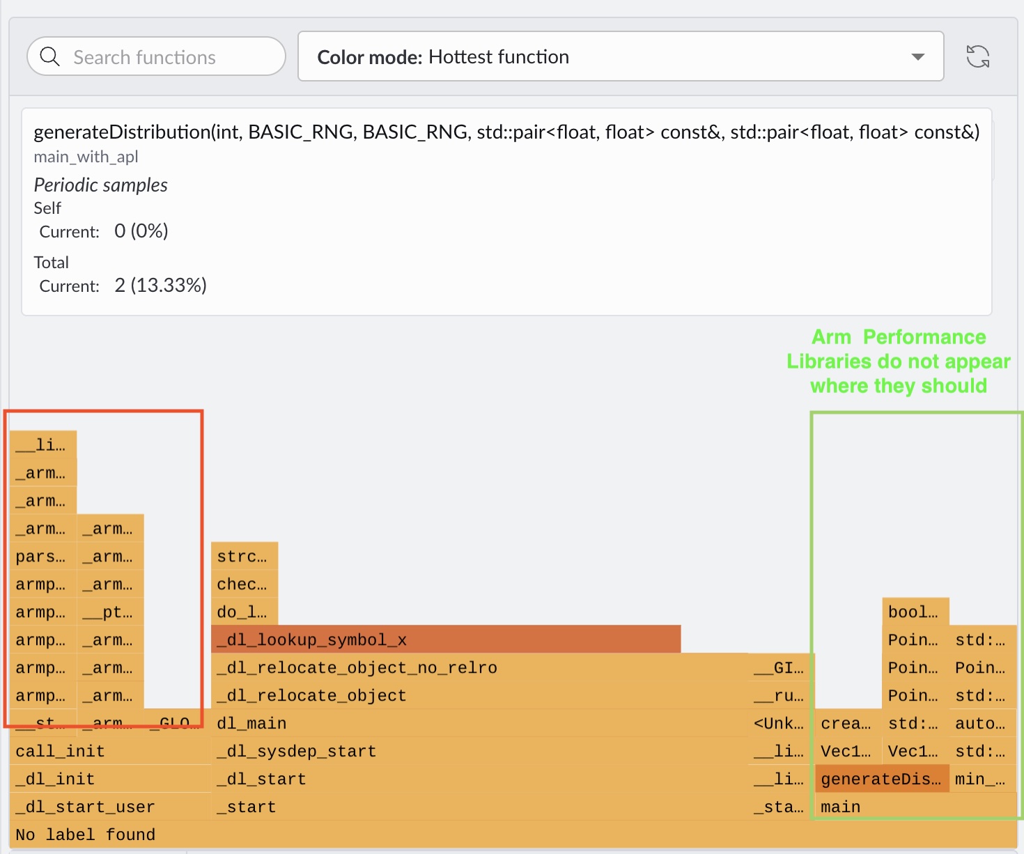
The flame graph shows main, but Arm Performance Libraries functions (including OpenRNG) don’t appear above it. Instead, most samples are attributed to dynamic loader functions (for example, _dl_*), which indicates missing symbol resolution. This often happens on Linux when pre-built shared libraries (*.so) don’t include debug symbols. The profiler can’t resolve internal library calls, so stacks appear truncated.
To fix this, rebuild OpenRNG from source with debug information enabled (for example, -g), so the library functions show up correctly above main.
Clone and build OpenRNG from the project root with debug symbols enabled:
git clone https://gitlab.arm.com/libraries/openrng.git && cd openrng
cmake -S . -B build -DCMAKE_BUILD_TYPE=Debug -DCMAKE_INSTALL_PREFIX=$PWD/install
cmake --build build -j $(nproc -1)
cmake --install build
cd ..
From the project root, compile the debug binary:
g++ --std=c++20 -g -O0 \
  src/main.cpp src/vec1d.cpp src/point.cpp src/rectangle.cpp src/export_data.cpp \
  -DUSE_ARMPL=1 \
  -I./include \
  -I./openrng/install/include \
  -I${ARMPL_DIR}/include \
  -L./openrng/install/lib64 \
  -L${ARMPL_DIR}/lib \
  -lopenrng -lamath -lm \
  -Wl,-rpath,$PWD/openrng/install/lib64 \
  -Wl,-rpath,${ARMPL_DIR}/lib \
  -o ./build/debug_openrng
OpenRNG uses the CMake build system. As an alternative, you can update your CMake configuration to fetch from the third-party library. The direct command is used here primarily for convenience.
From Performix, run the code hotspot recipe and target the ./build/debug_openrng binary. When the run completes, Performix displays the flame graph:
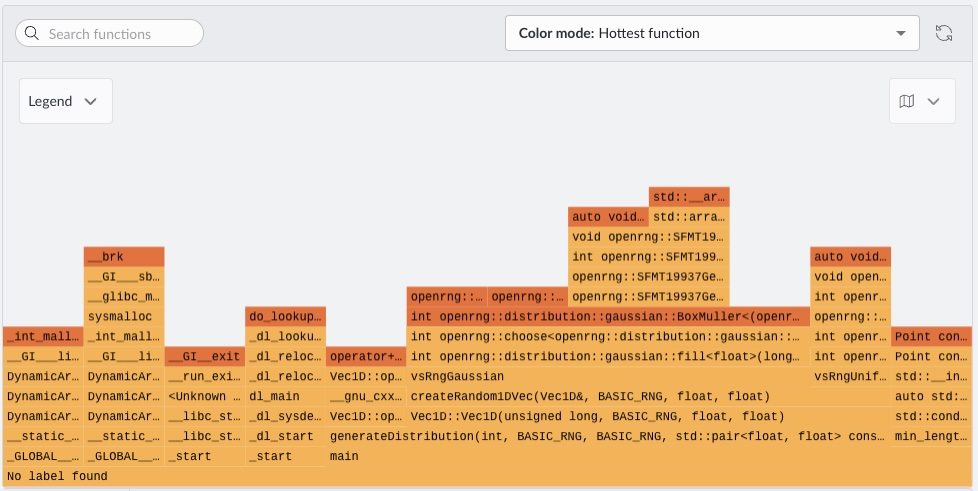
You can now correctly see the OpenRNG frames appearing above your calling functions. Because hotspots are identified through periodic sampling, the measurements provide limited direct insight into exact wall-clock time.
What you’ve accomplished and what’s next
In this section, you:
- Replaced the standard library random generation path with the OpenRNG vector API from Arm Performance Libraries
- Built and ran the accelerated executable
- Profiled the accelerated binary with Arm Performix
- Resolved missing symbol attribution by rebuilding OpenRNG from source with debug symbols
Next, you’ll measure the speedup of the hot function and examine how the improvement varies across different data sizes.