Run inference and evaluate the model

Objective

In this section, you’ll validate the digit recognizer by running inference on the validation dataset using both the PyTorch checkpoint and the exported ONNX model. Verify that PyTorch and ONNX Runtime produce consistent results, analyze class-level behavior using a confusion matrix, and generate visual diagnostics for debugging and documentation. This acts as a final verification checkpoint before integrating the model into the full OpenCV-based Sudoku processing pipeline.

Before introducing geometric processing, grid detection, and perspective correction, it is important to confirm that the digit recognizer works reliably in isolation. By validating inference and analyzing errors at the digit level, we ensure that any future issues in the end-to-end system can be attributed to image processing or geometry rather than the classifier itself.

Inference and Evaluation Script

Create a new file named 04_Test.py and paste the script below into it. This script evaluates the digit recognizer in a way that closely mirrors deployment conditions. It compares PyTorch and ONNX Runtime inference, measures accuracy on the validation dataset, and generates visual diagnostics that reveal both strengths and remaining failure modes of the model.

    

        
        
import os, numpy as np, torch
from torchvision import datasets, transforms
from torch.utils.data import DataLoader
from tqdm import tqdm
import matplotlib.pyplot as plt

from digitnet_model import DigitNet

DATA_DIR = "data"
ARTI_DIR = "artifacts"
os.makedirs(ARTI_DIR, exist_ok=True)

ONNX_PATH = os.path.join(ARTI_DIR, "sudoku_digitnet.onnx")  # fp32

# Same normalization as training (and force grayscale → 1 channel)
tfm_val = transforms.Compose([
    transforms.Grayscale(num_output_channels=1),
    transforms.ToTensor(),
    transforms.Normalize((0.5,), (0.5,))
])
val_ds = datasets.ImageFolder(os.path.join(DATA_DIR, "val"), transform=tfm_val)
val_loader = DataLoader(val_ds, batch_size=512, shuffle=False, num_workers=0)

DIGIT_NAMES = [str(i) for i in range(10)]  # 0 = blank, 1..9 = digits


def evaluate_pytorch(model, loader):
    model.eval()
    correct = total = 0
    with torch.no_grad():
        for x, y in loader:
            pred = model(x).argmax(1)
            correct += (pred == y).sum().item()
            total   += y.numel()
    return correct / total if total else 0.0


def confusion_matrix_onnx(onnx_model_path, loader):
    import onnxruntime as ort
    sess = ort.InferenceSession(onnx_model_path, providers=["CPUExecutionProvider"])
    mat = np.zeros((10, 10), dtype=np.int64)
    total = 0
    correct = 0
    for x, y in tqdm(loader, desc="ONNX eval"):
        # x: torch tensor [N,1,28,28] normalized to [-1,1]
        inp = x.numpy().astype(np.float32)
        logits = sess.run(["logits"], {"input": inp})[0]  # [N,10]
        pred = logits.argmax(axis=1)
        y_np = y.numpy()
        for t, p in zip(y_np, pred):
            mat[t, p] += 1
        correct += (pred == y_np).sum()
        total   += y_np.size
    acc = float(correct) / float(total) if total else 0.0
    return acc, mat


def plot_confusion_matrix(cm, classes=DIGIT_NAMES, normalize=False, title="Confusion matrix", fname=None):
    """Plot confusion matrix. If normalize=True, rows sum to 1."""
    cm_plot = cm.astype("float")
    if normalize:
        row_sums = cm_plot.sum(axis=1, keepdims=True) + 1e-12
        cm_plot = cm_plot / row_sums

    plt.figure(figsize=(6, 5))
    plt.imshow(cm_plot, interpolation="nearest")
    plt.title(title)
    plt.colorbar()
    tick_marks = np.arange(len(classes))
    plt.xticks(tick_marks, classes)
    plt.yticks(tick_marks, classes)

    # Label each cell
    thresh = cm_plot.max() / 2.0
    for i in range(cm_plot.shape[0]):
        for j in range(cm_plot.shape[1]):
            txt = f"{cm_plot[i, j]:.2f}" if normalize else f"{int(cm_plot[i, j])}"
            plt.text(j, i, txt,
                     horizontalalignment="center",
                     verticalalignment="center",
                     fontsize=7,
                     color="white" if cm_plot[i, j] > thresh else "black")

    plt.ylabel("True label")
    plt.xlabel("Predicted label")
    plt.tight_layout()
    if fname:
        plt.savefig(fname, dpi=150)
        print(f"Saved: {fname}")
    plt.show()


def sample_predictions_onnx(onnx_path, dataset, k=24, seed=0):
    """Show a grid of sample predictions (mix of correct and misclassified)."""
    import onnxruntime as ort
    rng = np.random.default_rng(seed)
    sess = ort.InferenceSession(onnx_path, providers=["CPUExecutionProvider"])

    # Over-sample candidates then choose some wrong + some right
    idxs = rng.choice(len(dataset), size=min(k * 2, len(dataset)), replace=False)
    imgs, ys, preds = [], [], []

    for i in idxs:
        x, y = dataset[i]  # x: [1,28,28] after transforms; y: int
        x_np = x.unsqueeze(0).numpy().astype(np.float32)  # [1,1,28,28]
        logits = sess.run(["logits"], {"input": x_np})[0]  # [1,10]
        p = int(np.argmax(logits, axis=1)[0])
        imgs.append(x.squeeze(0).numpy())  # [28,28]
        ys.append(int(y))
        preds.append(p)

    mis_idx = [i for i, (t, p) in enumerate(zip(ys, preds)) if t != p]
    cor_idx = [i for i, (t, p) in enumerate(zip(ys, preds)) if t == p]
    picked = (mis_idx[:k // 2] + cor_idx[:k - len(mis_idx[:k // 2])])[:k]
    if not picked:  # fallback
        picked = list(range(min(k, len(imgs))))

    # Plot grid
    import math
    cols = 8
    rows = math.ceil(len(picked) / cols)
    plt.figure(figsize=(cols * 1.6, rows * 1.8))
    for j, idx in enumerate(picked):
        plt.subplot(rows, cols, j + 1)
        plt.imshow(imgs[idx], cmap="gray")
        t, p = ys[idx], preds[idx]
        title = f"T:{t} P:{p}"
        color = "green" if t == p else "red"
        plt.title(title, color=color, fontsize=9)
        plt.axis("off")
    plt.tight_layout()
    out = os.path.join(ARTI_DIR, "samples_grid.png")
    plt.savefig(out, dpi=150)
    print(f"Saved: {out}")
    plt.show()

def main():
    # Optional: evaluate the best PyTorch checkpoint for reference
    pt_ckpt = os.path.join(ARTI_DIR, "digitnet_best.pth")
    if os.path.exists(pt_ckpt):
        model = DigitNet()
        model.load_state_dict(torch.load(pt_ckpt, map_location="cpu"))
        pt_acc = evaluate_pytorch(model, val_loader)
        print(f"PyTorch val acc: {pt_acc:.4f}")
    else:
        print("No PyTorch checkpoint found; skipping PT eval.")

    # Evaluate ONNX fp32
    if os.path.exists(ONNX_PATH):
        acc, cm = confusion_matrix_onnx(ONNX_PATH, val_loader)
        print(f"ONNX fp32 val acc: {acc:.4f}")
        print("Confusion matrix (rows=true, cols=pred):\n", cm)

        # Plots: counts + normalized
        plot_confusion_matrix(cm, normalize=False,
                              title="ONNX fp32 – Confusion (counts)",
                              fname=os.path.join(ARTI_DIR, "cm_fp32_counts.png"))
        plot_confusion_matrix(cm, normalize=True,
                              title="ONNX fp32 – Confusion (row-normalized)",
                              fname=os.path.join(ARTI_DIR, "cm_fp32_norm.png"))

        # Sample predictions grid
        try:
            sample_predictions_onnx(ONNX_PATH, val_ds, k=24)
        except Exception as e:
            print("Sample grid skipped:", e)
    else:
        print("Missing ONNX model:", ONNX_PATH)

if __name__ == "__main__":
    main()

    

The script first loads the validation dataset using the same preprocessing pipeline as training, including forced grayscale conversion to ensure a single input channel. It then optionally evaluates the best PyTorch checkpoint (digitnet_best.pth) to establish a reference accuracy.

Next, the exported ONNX model (sudoku_digitnet.onnx) is loaded using ONNX Runtime and evaluated in batches. Because the model was exported with a dynamic batch dimension, inference can be performed efficiently on larger batches, which is representative of how the model will be used later in the pipeline.

The script expects two things from the earlier steps:

1. A validation dataset stored under data/val/0..9/…
2. A trained model exported in previous step and stored under artifacts/
   • artifacts/digitnet_best.pth (optional, PyTorch weights)
   • artifacts/sudoku_digitnet.onnx (required, ONNX model)

When you run the script, it first loads the validation dataset using the same preprocessing as training, including forcing grayscale so the input has a single channel. It then optionally evaluates the PyTorch checkpoint to provide a reference accuracy. After that, it runs batched inference with ONNX Runtime, computes an overall accuracy, and builds a confusion matrix (true class vs predicted class) that reveals which digits are being confused.

In addition to printing accuracy metrics, the script generates two types of diagnostic outputs:

1. Confusion matrix visualizations, saved as:
   • artifacts/cm_fp32_counts.png (raw counts)
   • artifacts/cm_fp32_norm.png (row-normalized)
2. A grid of example predictions, saved as: *artifacts/samples_grid.png

These artifacts provide both quantitative and qualitative insight into model performance.

In the sample grid, each tile shows one crop together with its True label (T:) and Predicted label (P:), with correct predictions highlighted in green and mistakes highlighted in red. This makes it easy to quickly verify that the classifier behaves sensibly and to spot remaining failure modes.

Running the script

Before running the evaluation script, install matplotlib for visualization:

    

        
        
pip install matplotlib

    

Run the evaluation script:

    

        
        
python3 04_Test.py

    

The PyTorch and ONNX accuracies should match very closely, confirming that the export process preserved model behavior.

    

        
        
python3 04_Test.py 
PyTorch val acc: 0.9928
ONNX eval: 100%|███████████████████████████████████████████████████████████| 32/32 [00:01<00:00, 21.06it/s]
ONNX fp32 val acc: 0.9928
Confusion matrix (rows=true, cols=pred):
 [[12623     7     0     0     0     0     0     0     0     0]
 [    0   420     0     0     0     0     0     0     0     0]
 [    0     0   331     0     4     0     1     0     0     0]
 [    0     1     0   332     0     1     0     0     0     0]
 [    0     0     0     0   460     0     0     0     0     0]
 [    0     1     0     1     0   486     2     0     0     0]
 [    1     0     0     0     0    19   387     0     1     2]
 [    0     1     0     0     0     0     0   375     0     0]
 [    0     0     0     0     0     6    27     0   297    10]
 [    0     1     0     0     0    14    10     0     7   372]]
Saved: artifacts/cm_fp32_counts.png

    

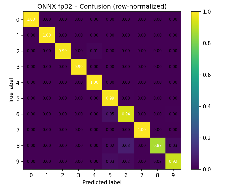
The confusion matrix provides more insight than a single accuracy number. Each row corresponds to the true class, and each column corresponds to the predicted class. A strong diagonal indicates correct classification. In this output, blank cells (class 0) are almost always recognized correctly, while the remaining errors occur primarily between visually similar printed digits such as 6, 8, and 9.

This behavior is expected and indicates that the model has learned meaningful digit features. The remaining confusions are rare and can be addressed later through targeted augmentation or higher-resolution crops if needed.

What you’ve learned and what’s next

In this section, you validated the digit recognizer by running inference on the validation dataset using both PyTorch and ONNX Runtime, confirmed that both produce consistent results (99.28% accuracy), and analyzed class-level behavior using confusion matrices and sample prediction grids. The diagnostic outputs revealed that the model performs reliably, with rare confusions limited to visually similar digits.

Next, you’ll integrate the validated ONNX model into the full Sudoku image-processing pipeline using OpenCV to detect grids, rectify perspective, segment cells, and perform batched inference to reconstruct and solve complete puzzles.