Understand YOLOX and KleidiCV in the detection pipeline

Understand the components of the pipeline

You’ll deploy a YOLOX object detection application on an arm64 Linux board and measure its image operations and full preprocessing latency. You’ll compare two OpenCV builds: a baseline without KleidiCV and a KleidiCV build using its default dispatch policy. A Radxa Orion O6 running 64-bit Debian is one suitable platform.

The application combines four components:

• YOLOX is the object detection model.
• Open Neural Network Exchange (ONNX) is the file format that’s used to store the trained model.
• OpenCV deep neural network (DNN) loads the ONNX file and runs the neural network.
• KleidiCV accelerates supported OpenCV image-processing operations on Arm CPUs.

What YOLOX is

YOLOX is a pretrained YOLOX-S object detection model from OpenCV Zoo in the ONNX format that you’ll run inference on. Trained on the Common Objects in Context (COCO) dataset, YOLOX recognizes 80 object classes. It predicts a bounding box, class, and confidence score for each detected object.

Understand the image-processing pipeline

The application processes the image in these stages:

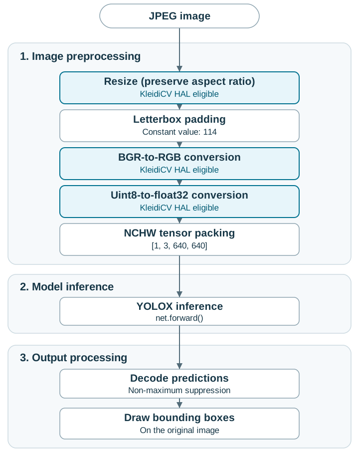YOLOX processing stages and KleidiCV-eligible operations

Non-maximum suppression removes duplicate detections before the application draws bounding boxes.

The letterbox operation resizes the image while preserving its aspect ratio and pads the unused area so that the result is 640 x 640, which is the YOLOX input size. The application then converts the OpenCV blue-green-red (BGR) image to red-green-blue (RGB). It changes the element type from unsigned 8-bit integers to 32-bit floating-point values. Pixel values remain in the 0 to 255 range expected by this YOLOX model.

OpenCV packs the prepared image into a tensor with this shape:

    

        
        
[1, 3, 640, 640]

    

The tensor represents the following dimensions:

• A batch size (N) of one image
• Three color channels (C)
• A height (H) of 640 pixels
• A width (W) of 640 pixels

Understand where KleidiCV is used

OpenCV integrates KleidiCV through its Hardware Acceleration Layer (HAL), so you can continue to call standard OpenCV functions. Acceleration depends on the build configuration, operation parameters, data type, and CPU features.

The application uses explicit OpenCV image-processing calls so that their costs can be measured separately:

    

        
        
cv::resize(image, resized, resizedSize, 0.0, 0.0, cv::INTER_LINEAR);
cv::copyMakeBorder(resized, padded, 0, bottom, 0, right,
                   cv::BORDER_CONSTANT, cv::Scalar::all(114));
cv::cvtColor(padded, rgb, cv::COLOR_BGR2RGB);
rgb.convertTo(floatImage, CV_32F);

    

The final blobFromImage() call only packs the tensor and doesn’t resize, swap channels, or scale values. Tensor packing belongs to OpenCV DNN, not the KleidiCV HAL.

KleidiCV doesn’t directly run the neural network. The OpenCV DNN call remains:

    

        
        
network.setInput(blob);
network.forward(outputs, network.getUnconnectedOutLayersNames());

    

The benchmark distinguishes two preprocessing metrics:

• Image operations subtotal (primary): Includes resizing, BGR-to-RGB conversion, and uint8-to-float32 conversion. These operations are eligible for KleidiCV HAL acceleration.
• Full preprocessing: Includes the three image operations as well as padding and tensor packing.

Individual preprocessing operations and DNN inference are also timed separately.

What you’ve learned and what’s next

You’ve identified the role of each component and the explicit preprocessing, inference, and output stages of the application.

Next, you’ll build matching baseline and KleidiCV installations to measure preprocessing and pipeline behavior.