Explore SME matrix operations with interactive visualizations
Introduction
Explore the ZA tile layout
Transpose a 32-bit matrix in place with ZA
Transpose a matrix with an incomplete edge
Multiply matrices with vector outer products
Transpose and pack matrix A
Pad matrix B to the ZA tile width
Trace packed GEMM through ZA
Compare a GEMM with gather loads
Interleave matrix A
Trace GEMM with interleaved matrix A
Next Steps
Explore SME matrix operations with interactive visualizations
Introduction
Explore the ZA tile layout
Transpose a 32-bit matrix in place with ZA
Transpose a matrix with an incomplete edge
Multiply matrices with vector outer products
Transpose and pack matrix A
Pad matrix B to the ZA tile width
Trace packed GEMM through ZA
Compare a GEMM with gather loads
Interleave matrix A
Trace GEMM with interleaved matrix A
Next Steps
Follow a GEMM with packed and padded inputs
This General Matrix Multiplication (GEMM) visualization multiplies matrix A (10 x 4) and matrix B (4 x 10), storing the resulting 10 x 10 matrix in Output Matrix Data.
You’ve seen in the previous visualizations how matrix A is transposed and packed, and how matrix B is padded. This packed 32-bit GEMM visualization starts with transposed and packed matrix A data and padded matrix B data already in memory.
The visualization processes horizontal blocks of three ZA tiles at a time, accumulating four partial results for each tile. Next, it writes the four rows of completed results to Output Matrix Data. It then resets the ZA tiles to zero before calculating three tiles for the next four rows.
The visualization stores the results and resets the tiles again to calculate the last three tiles, which cover the final two rows. In total, it processes nine tiles of matrix data.
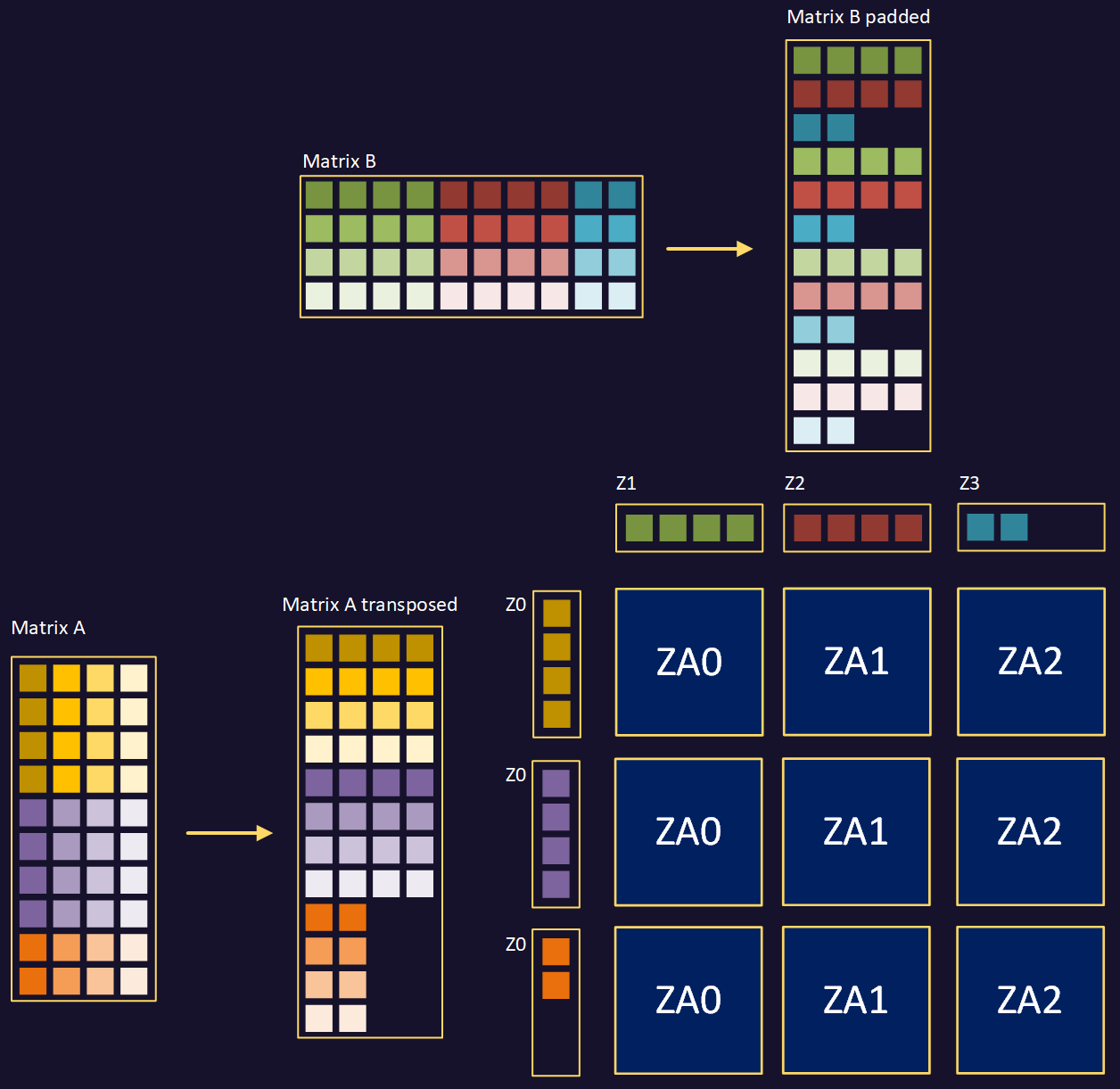 GEMM using packed transposed matrix A and padded matrix B
Why use a linear arrangement of three tiles
For large matrices, the most efficient arrangement is to process four tiles at a time, arranged in a 2 x 2 block. This requires four vector loads per four tiles of partial results.
This visualization processes three tiles at a time arranged in a 1 x 3 horizontal block. This arrangement requires four vector loads per three tiles of partial results. For a large matrix, it would be slightly less efficient than 2 x 2. However, this visualization uses a small matrix of size 10 x 10.
Consider Scalable Vector Length of 128 bits with 32-bit data element size. Using a 2 x 2 tile arrangement for a 10 x 10 matrix would require four passes. Using a 1 x 3 tile arrangement requires only three passes. For small matrices whose dimensions are known at compile time, the 2 x 2 configuration is sometimes outperformed by other tiling arrangements.
For larger scalable vector lengths, the calculus can change. For Scalable Vector Length of 256 bits, the 2 x 2 configuration would require only one pass. However, the 1 x 3 configuration would require two passes.
In this visualization, the code is functionally correct on all devices regardless of Scalable Vector Length. However, it’s optimized for devices with scalable vector length equal to 128 bits.
Trace packed GEMM loads and ZA accumulation
To keep this Learning Path open while exploring, open the GEMM visualization in a separate browser tab. Move the tab to a separate window to view the visualization and Learning Path side by side.
Follow the data from input through accumulation and storage. The following table summarizes how the visualization processes the first three tile-sized blocks, corresponding to the first four rows of input matrix data:
| Stage | Number of steps | Operation |
|---|---|---|
| Load the first row | 4 | Load the first row of A Packed Data into Z0 and the first row of B Padded Data into Z1–Z3. |
| Calculate the outer products | 3 | Calculate the matrix outer products in ZA0–ZA2. |
| Process the second row | 7 | Load the second row of A Packed Data into Z0 and the second row of B Padded Data into Z1 - Z3. Accumulate the outer products in ZA0–ZA2. |
| Process the remaining rows | 14 | Repeat the load and accumulation operations for rows three and four. |
| Store the results | 12 | Store rows of ZA0–ZA2 in Output Matrix Data. |
| Clear the tiles | 3 | Zero the ZA0–ZA2 tiles to prepare for the next block of four rows. |
Processing subsequent blocks
After clearing ZA0–ZA2, the algorithm moves down by one tile-sized block in A Packed Data. It returns to the leftmost column of B Padded Data.
Processing the next three tile-sized blocks that correspond to the next four rows shown purple in the top diagram, requires another 43 steps:
| Stage | Number of steps | Operation |
|---|---|---|
| Calculate outer products | 28 | Load data and calculate outer products for four rows |
| Store to memory | 12 | Store the results to Output Matrix Data |
| Clear the ZA tiles | 3 | Clear the ZA tiles ready for the next blocks |
Processing the final three tile-sized blocks that correspond to the last two rows shown orange in the top diagram, requires 34 steps:
| Stage | Number of steps | Operation |
|---|---|---|
| Calculate outer products | 28 | Load data and calculate outer products for four rows |
| Store to memory | 6 | Store the results to Output Matrix Data. Only six steps because just two rows remain. |
Why this approach is better than scalar processing
The visualization calculates 100 elements of the output matrix with only 120 instructions, excluding loop control instructions. This is an efficiency of 0.83 output elements per instruction.
With scalar processing, excluding loop control instructions, each output element would require the following instructions:
- Eight load instructions
- Four multiply-accumulate instructions
- One store instruction
This is 13 instructions, which is an efficiency of 0.08 output elements per instruction.
Consider a larger matrix of 12 x 12. The Scalable Matrix Extension (SME) implementation would take the same 120 cycles to process 144 output elements. This is 1.44 output elements per instruction. The scalar implementation would produce the same 0.08 output elements per instruction.
For larger Scalable Vector Length, the efficiency is much higher. Every time the Scalable Vector Length doubles, the efficiency quadruples for large matrices. For small matrices, edge effects can limit these gains. For example, for Scalable Vector Length of 512 bits, each ZA tile is 16 x 16 elements of 32-bit data. This is 256 elements in total. The 10 x 10 matrix is only 100 elements. It therefore uses just under 40% of the available throughput of one tile.
What you’ve learned and what’s next
You’ve traced loads, outer product accumulations, and stores in a GEMM that uses prepared operands. The visualization models data movement. It doesn’t measure performance or prove which instructions a processor runs.
For executable code built around the same outer-product idea, see matrix multiplication using SME2 intrinsics in C . The code uses its own FP32 data layout and instruction sequence.
Next, you’ll compare a version that loads matrix A in a different layout.