Explore SME matrix operations with interactive visualizations
Introduction
Explore the ZA tile layout
Transpose a 32-bit matrix in place with ZA
Transpose a matrix with an incomplete edge
Multiply matrices with vector outer products
Transpose and pack matrix A
Pad matrix B to the ZA tile width
Trace packed GEMM through ZA
Compare a GEMM with gather loads
Interleave matrix A
Trace GEMM with interleaved matrix A
Next Steps
Explore SME matrix operations with interactive visualizations
Introduction
Explore the ZA tile layout
Transpose a 32-bit matrix in place with ZA
Transpose a matrix with an incomplete edge
Multiply matrices with vector outer products
Transpose and pack matrix A
Pad matrix B to the ZA tile width
Trace packed GEMM through ZA
Compare a GEMM with gather loads
Interleave matrix A
Trace GEMM with interleaved matrix A
Next Steps
Matrix multiplication recap
When you multiply input matrix A by input matrix B, you get a resulting matrix C. Matrix C is the sum of products of pairs of values from the rows of A and the columns of B.
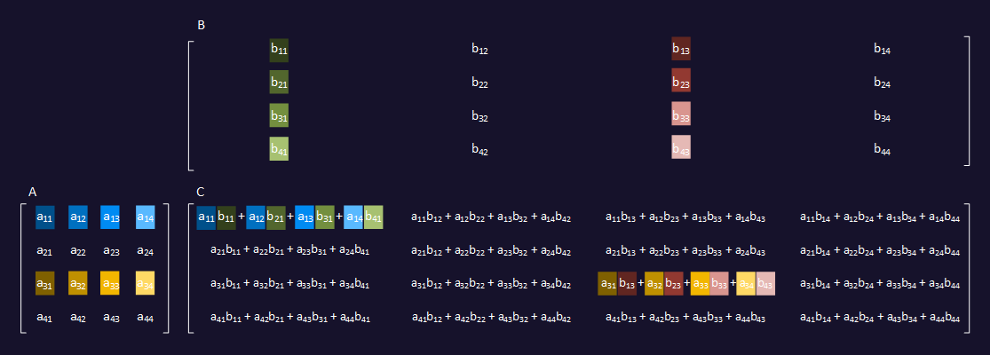 Scalar multiplication
Vectorize matrix multiplication
Calculating the successive terms of each element of matrix C isn’t a good candidate for two dimensional vectorization. Instead, decompose the operation to calculate partial results for many rows and columns at a time.
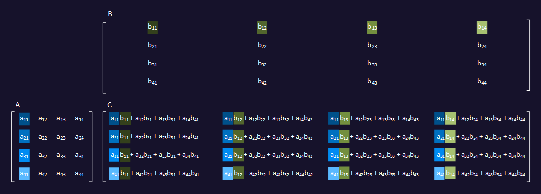 Vector first partial result
This is efficient because a Scalable Matrix Extension (SME) Matrix Outer Product instruction calculates all these values at the same time. It can accumulate the result by adding it to or subtracting it from the value that’s already in the ZA tile.
After completing this step, move on to the second partial result.
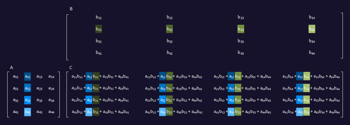 Vector second partial result
The pattern continues for the third partial result, using the third column of A and the third row of B.
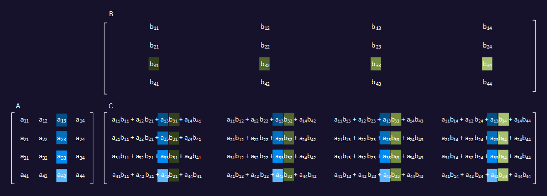 Vector third partial result
After you accumulate the fourth partial result, you’ve fully calculated the result values for 16 elements of the output matrix.
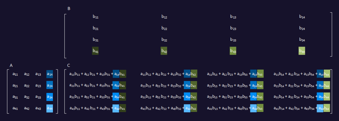 Vector fourth partial result
More results would have been calculated from the same number of instructions in the following circumstances:
- If smaller data types were used
- If the device used had a larger scalable vector length
Optimize memory access
The input matrix B is accessed sequentially, which is efficient. However, with input matrix A, you access columns of data whose elements are separated in memory by one row length. This is less efficient and can result in multiple cache misses, particularly if the row length is large. To avoid this, it’s preferable to transform the input matrix A data so that it can be read sequentially. Do this by transposing strips of the matrix. Each strip contains the same number of rows as the ZA tiles of the element size that you’re working with.
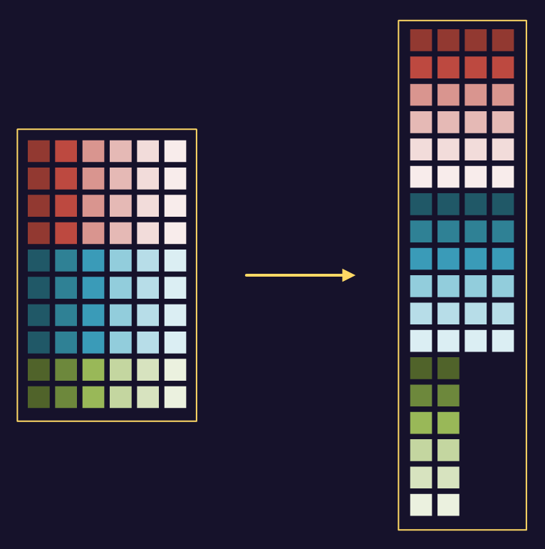 Transforming the input matrix A
It’s best if the input matrix data can naturally arise in this form. That way, there’s no computational cost to transform the data. If that isn’t possible, it might be desirable to manually transform the data.
Where the final strip doesn’t contain the same number of rows as the others, pad the missing rows with 0.
Use multiple ZA tiles
For data element size larger than 8 bits, there are multiple ZA tiles available. Use all of them to achieve the greatest data reuse and minimize memory system access.
In the diagram that follows, four tiles of results are processed at a time. Matrix B data is accessed sequentially from memory. Matrix A data is accessed as columns within horizontal strips, shown as a blue strip and a yellow strip. The height of each strip depends on the scalable vector length.
The ZA0 partial results are generated from an outer product of the blue and green data. The ZA1 partial results are generated from an outer product of the blue and red data. For the remaining tiles, you also need to load the yellow data. The ZA2 partial results are generated from an outer product of the yellow and green data. The ZA3 partial results are generated from an outer product of the yellow and red data.
As a result, the access pattern for matrix A is to alternate reading a column of blue data followed by a column of yellow data. Therefore, in addition to transposing strips of matrix A, an optimal arrangement involves interleaving the transposed rows from each strip.
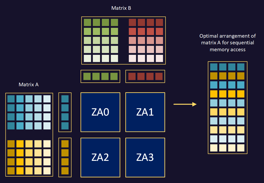 Transforming the input matrix A with interleave
Other tiling arrangements are possible. For example, you can process four tiles arranged horizontally, instead of two rows of two. However, this arrangement is slightly less efficient. This is because it would require five vector loads from memory for every four tiles of partial results processed. The two-by-two arrangement requires only four vector loads from memory per four tiles.
What you’ve learned and what’s next
You’ve reviewed how matrix multiplication works, and how it can be decomposed into vector operations. You’ve seen how matrix A input data can be transposed so that it’s accessed sequentially in memory. You’ve learned how to use multiple ZA tiles to increase data reuse and minimize memory system access.
Next, you’ll view a visualization that prepares matrix A for multiplication.